
Mastering VLOOKUP in Excel: A Step-by-Step Guide
If
you work with data in Excel, VLOOKUP is one of the most powerful and commonly
used functions. Whether you're analyzing sales reports, managing inventory, or
consolidating data from multiple sources, VLOOKUP can save you time and
effort.

VLOOKUP Function?
VLOOKUP (Vertical Lookup) is an Excel function that searches for a value in the first column of a table and returns a corresponding value from another column in the same row.
Syntax of VLOOKUP
=VLOOKUP(lookup_value, table_array, col_index_num, [range_lookup])
 |
| excel vlookup |
- lookup_value: The value you want to search for.
- table_array: The range of cells where Excel should look for the data.
- col_index_num: The column number (from the table) containing the return value.
- range_lookup (optional):
- TRUE` (or `1`) for approximate match (default).
- FALSE (or `0`) for exact match.
How to use the VLOOKUP function.
- Select a cell (H4)
- Type =VLOOKUP
- Double click the VLOOKUP command
- Select the cell where search value will be entered (H3)
- Type (,)
- Mark table range (A2:E21)
- Type (,)
- Type the number of the column, counted from the left (2)
- Type True (1) or False (0) (1)
- Hit enter
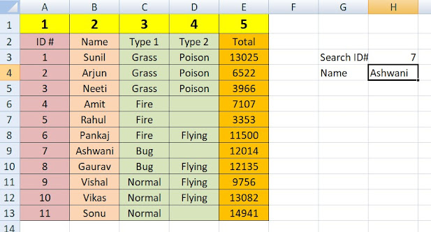
- Enter a value in the cell selected for the Lookup_value H3(7)
Let's have a look at an example!
Use the VLOOKUP function to find the Pokemon names based on their ID#:
 H4 is where the search result is displayed. In this case, the Pokemons names based on their ID#

VLOOKUP EXAMPLE1

VLOOKUP EXCEL
The range of the table is marked at table_array, in this example A2:E21.

 |
| VLOOKUP EXAMPLE1 |


An illustration for selecting col_index_number 2


Ok, so next - 1 (True) is entered as range_lookup. This is because the most left column has numbers only. If it was text, 0 (False) would have been used.
The function returns the #N/A value. This is because there have not been entered any value to the Search ID# H3.
Let us feed a value to it, type H3(7):
excel vlookup

إرسال تعليق